

New research documenting the melting of ice sheets in East Antarctica since the last ice age is providing crucial data for scientists to accurately project sea-level rises by the end of the 21st century.
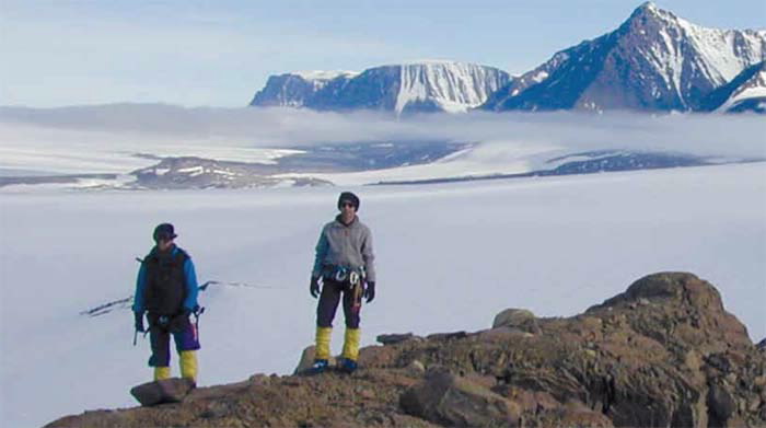 |
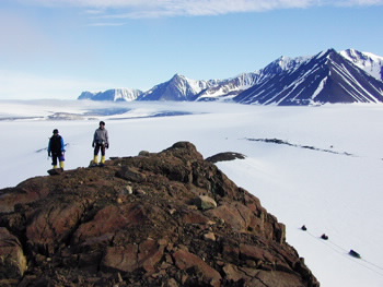
| View of the Prince Charles Mountain flanking the Lambert Glacier near Loewe Massif. |
Introduction
Current global climate models do not fully incorporate the contribution of Antarctic Ice Sheets to changes in sea level despite dramatic changes in the past. Projected sea-level rise by the end of the 21st century ranges from 20 to 60 centimetres, mainly attributed to the Antarctic Peninsula, Greenland and ocean thermal expansion.
During the last ice age, about 20,000-25,000 years ago, the sea-level was 120 metres lower and Antarctic ice volume three times larger than today. Hence, documenting the size and retreat rate of the East Antarctic Ice Sheet since the last ice age will allow a better understanding of ice-sheet dynamics, improve sensitivity to increasing warming and validate predictions of future sea-level change.
Using the new innovative technique of in situ cosmogenic radionuclide surface exposure dating, we can for the first time provide quantitative geochronological constraints on the variability and sensitivity of East Antarctic ice volume, suggesting that parts of the Ice Sheet respond more rapidly to global climate variability than previously assumed, and that East Antarctica was not responsible for a controversial dramatic pulse in sea-level rise of 20 metres 14,500 years ago.
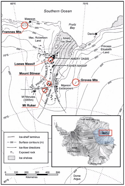 |
| Fig 1. Map of the 5 locations (red underline) in the Prince Charles-Lambert-Amery region where transported boulders and exposed bedrock were sampled for radionuclide analyses at the ANTARES AMS facility at ANSTO. The stippled area is floating Amery Ice Shelf; continuous numbered lines represent contours of altitude above sea level of today’s ice sheet surface. Inset shows full Antarctic continent with darker blue shaded region indicating the area of the ice sheet which drains through the Prince Charles-Lambert basin shown within the red rectangle. |
Tackling ice-volume changes of the East Antarctic Ice Sheet
The East Antarctic Ice Sheet holds enough ice to raise global sea level by ~60 metres, but because surface temperatures are well below freezing point, this ice is relatively stable, and thus unlikely to contribute significantly to sea level rise during the next few centuries.
Most of the contribution to sea level from melted ice occurs along the coastal perimeter of East Antarctica where the slow moving ice-sheet calves directly into the ocean and via large outlet glaciers which stream through deep and extensive basins that act like drainage channels. Little is known on the magnitude and rates of change of these two mechanisms.
As glaciers advance down a valley scouring and cutting bedrock they accumulate and transport debris, ranging in size from small cobbles to large boulders.
Moraines are piles of accumulated boulders which are deposited at the perimeter of a glacier when the advance ceases and it begins to retreat up a valley.
Moraines represent past ice limits and changes in climatic conditions. The boulders of such moraines deposited over the flanks of mountain ranges, which constrain the passage of outlet glaciers of the Antarctica ice sheet, form the basis of our study.
We used the mountain ranges that protrude above the ice sheet as ‘dipsticks’ to measure past ice-sheet elevation. By correlating exposure ages (i.e. boulder deposition age) of glacially transported boulders on a moraine with altitude, we can map the evolution of the ice sheet and quantify ice-volume changes as a function of time.
New cosmogenic exposure ages and field-based studies indicate that since the Last Glacial Maximum, increased atmospheric temperatures and coastal instability due to sea level increase causes icestreaming sections of the EAIS to respond more rapidly to global climate variability than previously assumed.
 |  |
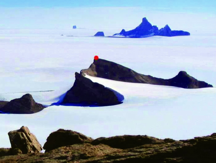 | 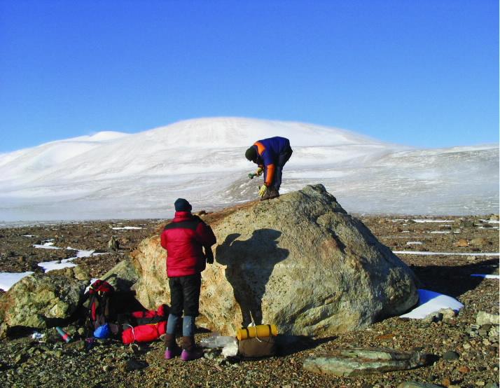 |
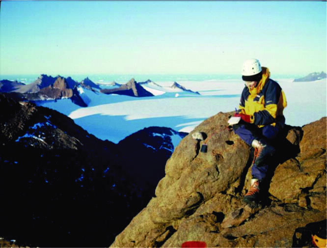
| Various photographs of sampling sites: (A) View of the Prince Charles Mountain flanking the Lambert Glacier near Loewe Massif. Light coloured rocks or cobbles contrast with the darkerlocal bedrock lithology. Two samples gave exposure ages of 18,500 and 17,400 years suggesting that at that time the surface of the Lambert glacier was about 300 metres higher than today. (B) Small cobble on the peak of Central Mason Range (1035 m above sea level and 330 metres above today’s ice surface) in Framnes Mountains, which gave an exposure age of 9500 years. Note the ocean coastline in background. (C) View of Groves Mountains looking south towards the centre of the East Antarctic Ice Sheet. These mountains protruding only 100-150 metres above the Ice Sheet are the most southern of any in the region. The reddot indicates one of the bedrock sample sites which gave an exposure age of about 2.5 million years indicating relatively little change of ice volume and hence a static ice-sheet surface. (D) An example of a very large boulder transported and deposited by the Lambert glacier. Samples for exposure dating are taken from the very uppermost flat surface of the boulder usually a few centimetres in thickness, by chisel and hammer. |
How do we measure cosmogenic exposure ages?
The radionuclides 10Be (T1/2=1.38 million years) and 26Al (0.70 million years) are produced in exposed surface rocks and within a metre or so of the Earth’s crust by the secondary cosmic ray flux (fast neutrons) which penetrate Earth’s atmosphere.
Despite ultra-low in situ production rates only five atoms of 10Be are produced each year per gram of rock.
The technique of Accelerator Mass Spectrometry (AMS) [1] using ANSTO’s ANTARES Facility can measure this tell-tale signal. As the concentration builds up over time with continued exposure to cosmic rays, in situ cosmogenic radionuclides act as nuclear clocks which measure an ‘exposure age’.
This technique has revolutionised our understating of changing landscapes and of continental glacial chronologies.
|
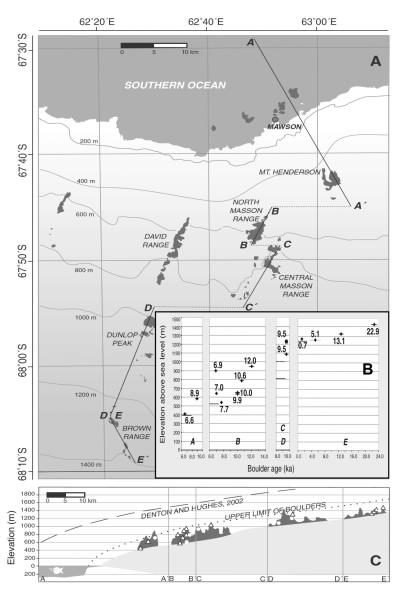
| Fig 3. (A) Map of Framnes Mountains, Mac.Robertson Land, near Mawson Station. Transect A-E traces the chain of mountains which act as elevation ‘dipsticks’ allowing past changes in ice sheet volume to be constrained. (B) Inset shows elevation against exposure age (in thousand years) for each mountain range labeled A to E in the transect. Dashed lines denote present day local ice sheet elevation at individual sections. For example, panel A (Mt. Henderson) shows ~200 m of ice sheet lowering occurred between ~8900 and 6600 years; panel B (North Masson Range) provides evidence for 350 m of ice sheet lowering between 12,000 and 7000 years. (C) Modelled ice sheet surface during the last ice age—compared to measured surface based on exposure age dating (dotted line represents upper limit of boulders with exposure ages). The measured profile suggests a much smaller ice sheet in the past (500-1000 metres thinner and ~10 km less in extension over the continental shelf). Also coastal ice sheet deglaciation commences at 13,000 years - about 1000-2000 years before Meltwater pulse-1a which has previously been attributed to Antarctic ice melt. |
Study region - Lambert Glacier and Prince Charles Mountains
We measured exposure ages of glacial boulders from three distinct regions of the EAIS that are characterised by vastly different modes of dynamical ice behaviour (see Fig. 1 in the image library at the end of this article).
- The Southern and Northern Prince Charles Mountains border the Lambert Glacier-Amery Ice Shelf region (Fig. 2A), which acts as an extensive ice-stream drainage basin extending ~800 km inland funnelling an estimated ~15% of East Antarctica’s ice onto the Amery Shelf. As an outlet glacier system rapidly conveying ice from the deep interior to the coast, it effectively propagates large ocean-atmospheric variability to regions of static ice-sheet frozen to its bed which otherwise would be decoupled from external forcing.
- The Framnes Mountains (Fig. 2B) near Mawson station are a string of localised coastal mountain peaks previously overridden by the EAIS, which today act as obstructive dipsticks protruding through the ice surface. At Framnes, the EAIS is slow and calves directly into the ocean; hence rising sea-level can unhinge basal ice-flow and change the rate of ice-sheet loss.
- The Groves Mountains (Fig. 2C), smaller in area and only 200 m above the present ice surface, is fully encircled by the EAIS to the south-east beyond the drainage contours of the Lambert Glacier. The Groves Mountains are considered to be the most isolated land-mass within the deep interior of the EAIS.
|
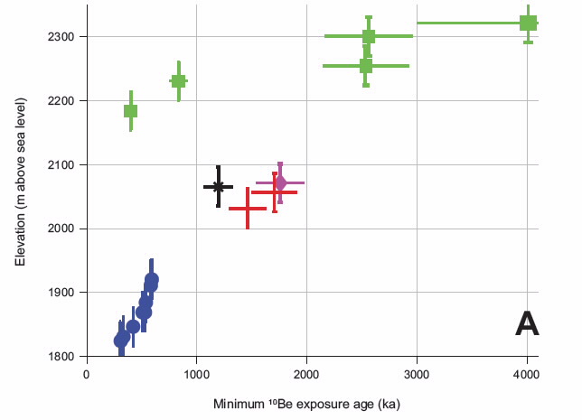
| Fig 4. Altitude vs exposure ages (ka is 1000 years) at Groves Mountains deep within the Ice Sheet interior. Exposure ages of the mountain peaks show a long-term stable ice-sheet surface which has altered by only about ~400 m in thickness over the past 3 million years. |
Exposure ages document ice-sheet volume changes
Our results indicate that after the last ice age, ice thickness in the Lambert Glacier ice-streaming region began to decrease 18,000 to 14,000 years ago [2,3].
At the adjacent regions of the Framnes Mountains, where the EAIS reaches the coastline, our exposure ages [4] indicate that the ice-sheet retreat commenced only at 13,000 years and continued to 6000-7000 years at which time the ice sheet stabilises [4] (Fig. 3B).
This phase of ice-volume reduction at Framnes occurred about 4000 - 6000 years later than registered by the Lambert Glacier. Earlier onset of deglaciation of drainage basins suggests a heightened sensitivity of the EAIS to climate variability.
Such effects are not included in any climate models.
In contrast to these short-term ice-volume changes, our exposure ages at Groves Mountains tells a far different story, varying in thickness by ~100 metres at each mountain ‘dipstick’ with a total ice-thickness reduction of ~300 metres compared to today’s ice surface in the past three million years – effectively a passive ice surface with little overall change during this time (Fig. 4).
Our exposure ages do not only provide dates, but also information on the spatial distribution of ice volume. By combining all ice limits traced out by the dated moraines across the Framnes region, we can reconstruct a picture of the dimensions of the coastal ice-sheet surface at the Last Glacial Maximum and thus predict how far it extended over the surrounding Southern Ocean (Fig. 3C).
Our surface reconstruction indicates an ice-sheet thickness only a few hundred metres thick and a few kilometres out to sea rather than predicted by some contemporary ice-sheet models which show ice 1000 metres thicker and tens of kilometres larger over the ocean.
Hence, we argue that there were only minor reductions in East Antarctic Ice Sheet thickness from 13,000 - 6000 years, a period during which northern hemisphere ice-sheets all but disappeared and sea levels rose by about 100 metres.
This discovery leads onto a second very exciting conclusion. Past sea-level records across global oceans document a continuous increasing sea-level totalling 120 metres from 20,000 years to about 6000 years ago.
This trend is punctuated by a dramatic short pulse of a 20 metre rise about 14,500 years ago called Meltwater Pulse-1a. Most scientists point at Antarctica as the only source of such a large volume of water. Our results indicate that ice-streaming melt occurred well before this pulse, and coastal ice-sheet melt initiated about 1000 to 2000 years after it.
Hence, we present a controversial conclusion that coastal EAIS retreat is not a contributor to Meltwater Pulse-1a because of a far smaller available ice volume and because coastal deglaciation postdates the pulse by 1000 - 2000 years.
We have shown that the EAIS does not respond uniformly both in space and time across all sectors to global climate variability. Our improved documentation of size and thickness of the EAIS at the Last Glacial Maximum, as well as comparison of retreat rates between coastal margins and drainage basins are essential input to improving ice-sheet modelling and predicting future sea-level rise.
Authors
David Fink1, Charles Mifsud1, Duanne White2, Kat Lilly3, Andrew Makintosh4, Derek Fabel5
1ANSTO, 2Macquarie University, 3University of Otago (NZ), 4Victoria University (NZ), 5University of Glasgow (UK)
References
- Tuniz, C., Bird, R., Fink, D., & Herzog, G. (1998). Accelerator Mass Spectrometry: Ultrasensitive Analysis for Global Science. Boca Raton, Florida, United States of America: CRC Press. 371p.
- White, D., Fink, D., & Gore, D., Cosmogenic nuclide evidence for enhanced sensitivity of an East Antarctic ice stream to change during the last deglaciation. Geology, 39(1), 23-26.
- Fink, D., McKelvey, B., Hambrey, M. J., Fabel, D., & Brown, R. (2006). Pleistocene deglaciation chronology of the Amery Oasis and Radok Lake, northern Prince Charles Mountains, Antarctica. Earth and Planetary Science Letters, 243(1-2), 229-243.
- Mackintosh, A., White, D., Fink, D., Gore, D. B., Pickard, J., & Fanning, P. C. (2007). Exposure ages from mountain dipsticks in Mac. Robertson Land, East Antarctica, indicate little change in ice-sheet thickness since the Last GlacialMaximum. Geology, 35(6), 551-554.
- Lilly, K., Fink, D., Fabel, D., & Lambeck, K. (2010). Pleistocene dynamics of the interior East Antarctic ice sheet. Geology, 38(8), 703-706.
Published: 04/06/2011